A Design Of Experiments Class
Introduction
This project is a quick analysis of the Design of Experiments class carried out in the Order and Chaos course, FSP-2021-2022, at SMI MAHE, Bangalore.
The methodology followed was that in A.J. Lawrance’s paper 1 describing a Statistics module based on the method of Design of Experiments. The inquiry relates to Short Term Memory (STM) among students.
Structure
The total number of students were 17. Eight Pairs of students were created randomly to create eight different Test tools for Short Term Memory testing.
The binary ( two - level ) variables/parameters that were used in the tests, were, following Lawrance:
- WL: Word List Length ( 7 and 15 words )
- SL: Syllables in the Words ( 2 and 5 syllables )
- ST: Study Time allowed for the Respondents ( 15 and 30 seconds )
Other parameters considered were a) Language b) Structure/Depiction of the Word Lists ( e.g. word clouds, matrices, columns…), c) Whether the words would be shown or read aloud, and d) whether the respondents had to speak out, or write down, the recollected words. These parameters were discussed and abandoned as too complex to mechanize, though they could have had an impact on the STM scores.
Hence a total of 8 Tests were created by 8 pairs of students, and each team tested the remaining 15 students ( Due to COVID restrictions, this testing was carried out entirely online on MS Teams, using individual breakout rooms for the Test Teams. )
The data were entered into a Google Sheet and the STM scores were converted to percentages so as to be comparable across WL.
The data was then “flattened” for each of the binary parameters; this was logical to do since for each parameter, the other two parameters were balanced out by the Test structure. For instance, for WL = 5, the SL and ST parameters used all the four combinations ( SL = 5, 15 ) and (ST = 15, 30 ). Hence the “common sense” analysis could proceed for each of the parameters individually. Joint effects were not considered for this preliminary class.
Data
## # A tibble: 60 × 6
##    syllable_2 syllable_5 study_time_15 study_time_30 list_length_7
##         <dbl>      <dbl>         <dbl>         <dbl>         <dbl>
##  1      0.714      0.571         0.714         0.714         0.714
##  2      0.429      0.571         0.429         0.571         0.429
##  3      0.571      0.714         0.571         0.571         0.571
##  4      0.714      1             0.714         0.571         0.714
##  5      0.714      1             0.714         1             0.714
##  6      0.714      0.857         0.714         0.714         0.714
##  7      0.571      0.571         0.571         0.571         0.571
##  8      0.571      0.714         0.571         0.571         0.571
##  9      0.571      0.857         0.571         1             0.571
## 10      0.571      1             0.571         0.429         0.571
## # ℹ 50 more rows
## # ℹ 1 more variable: list_length_15 <dbl>
The data has scores that have been combined into single columns for each setting for each of the parameters. For example, the column syllable_2 contains STM scores for all tests that used SL = 2-syllables in their tests. The Word Length WL and Study Time ST go through all their combinations in this column.
The other columns are constructed similarly.
Basic Plots
We will use Box Plots and Density Plots to compare the STM score distributions for each Parameter. To do this we need to pivot_longer the adjacent columns ( e.g. syllable_2 and syllable_5) and use these names as categorical variables:
Syllable Parameter SL
## # A tibble: 120 × 2
##    syllable   syl_scores
##    <chr>           <dbl>
##  1 syllable_2      0.714
##  2 syllable_5      0.571
##  3 syllable_2      0.429
##  4 syllable_5      0.571
##  5 syllable_2      0.571
##  6 syllable_5      0.714
##  7 syllable_2      0.714
##  8 syllable_5      1
##  9 syllable_2      0.714
## 10 syllable_5      1
## # ℹ 110 more rows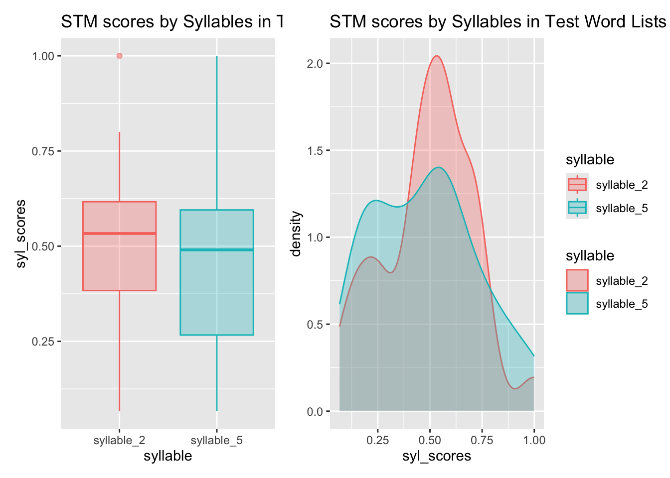
Study Time Parameter ST
## # A tibble: 120 × 2
##    study         study_scores
##    <chr>                <dbl>
##  1 study_time_15        0.714
##  2 study_time_30        0.714
##  3 study_time_15        0.429
##  4 study_time_30        0.571
##  5 study_time_15        0.571
##  6 study_time_30        0.571
##  7 study_time_15        0.714
##  8 study_time_30        0.571
##  9 study_time_15        0.714
## 10 study_time_30        1
## # ℹ 110 more rows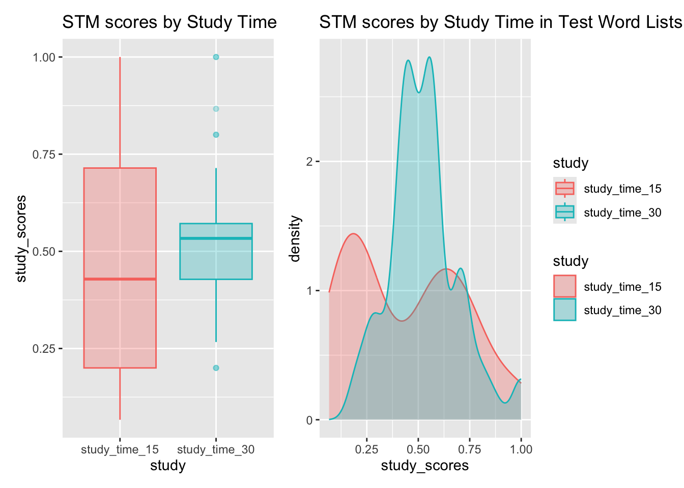
Word List Length Parameter WL
## # A tibble: 120 × 2
##    list           list_scores
##    <chr>                <dbl>
##  1 list_length_7       0.714
##  2 list_length_15      0.267
##  3 list_length_7       0.429
##  4 list_length_15      0.2
##  5 list_length_7       0.571
##  6 list_length_15      0.0667
##  7 list_length_7       0.714
##  8 list_length_15      0.133
##  9 list_length_7       0.714
## 10 list_length_15      0.2
## # ℹ 110 more rows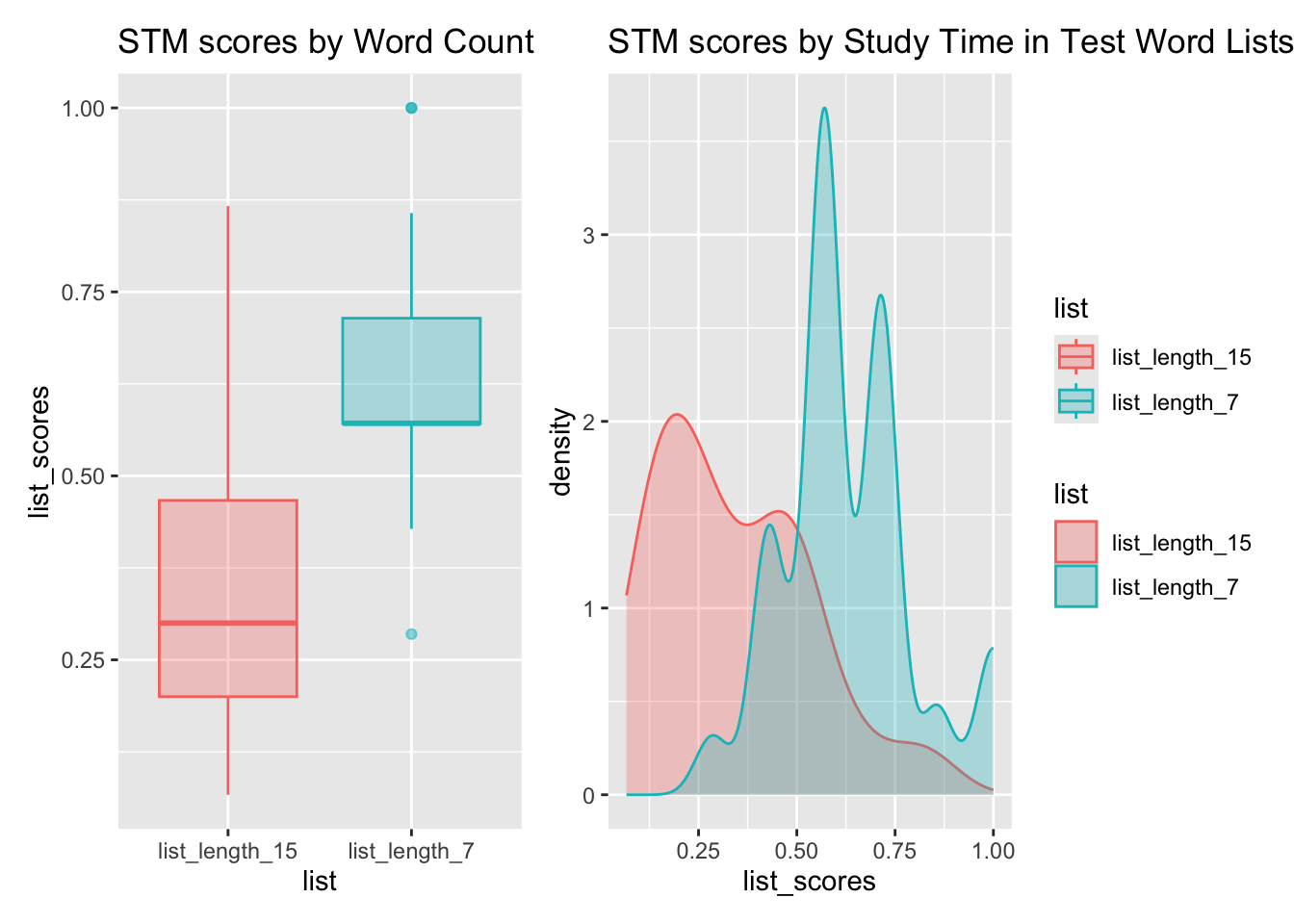
Preliminary Observations
Clearly, based on visual inspection of the Plots, the Word Count seems to have a large effect on STM Test Scores, with fewer words ( 7 ) being easier to recall. Study Time ( 15 and 30 seconds ) also seems to have a more modest positive effect on STM scores, while Syllable Count ( 2 or 5 syllables ) seems to have a modest negative effect on STM scores.
Analysis
We wish to establish the significance of the effect size due to each of the Parameters. Already from the Density Plots, we can see that none of the scores are normally distributed. A quick Shapiro-Wilkes Test for each of them confirms that the scores are not normally distributed.
Hence we go for a Permutation Test to check for significance of effect.
On the other hand, as remarked in Ernst2, the non-parametric permutation test can be both exact and also intuitively easier for students to grasp, as I can testify from direct observation in this class. There is no need to discuss sampling distributions and means, t-tests and the like. Permutations are easily executed in R, using packages such as mosaic3.
##
## 	Shapiro-Wilk normality test
##
## data:  stm$syllable_2
## W = 0.95508, p-value = 0.02716##
## Shapiro-Wilk normality test
##
## data: stm$syllable_5
## W = 0.95321, p-value = 0.02211##
## Shapiro-Wilk normality test
##
## data: stm$study_time_15
## W = 0.9068, p-value = 0.0002348##
## Shapiro-Wilk normality test
##
## data: stm$study_time_30
## W = 0.95539, p-value = 0.0281##
## Shapiro-Wilk normality test
##
## data: stm$list_length_7
## W = 0.90542, p-value = 0.0002085##
## Shapiro-Wilk normality test
##
## data: stm$list_length_15
## W = 0.92806, p-value = 0.001645Permutation Tests
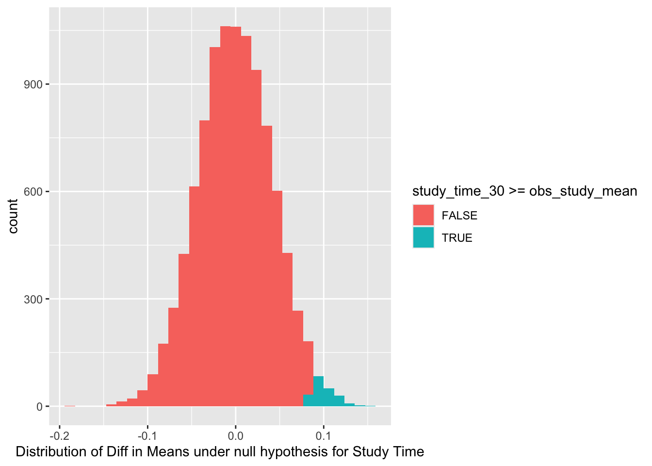
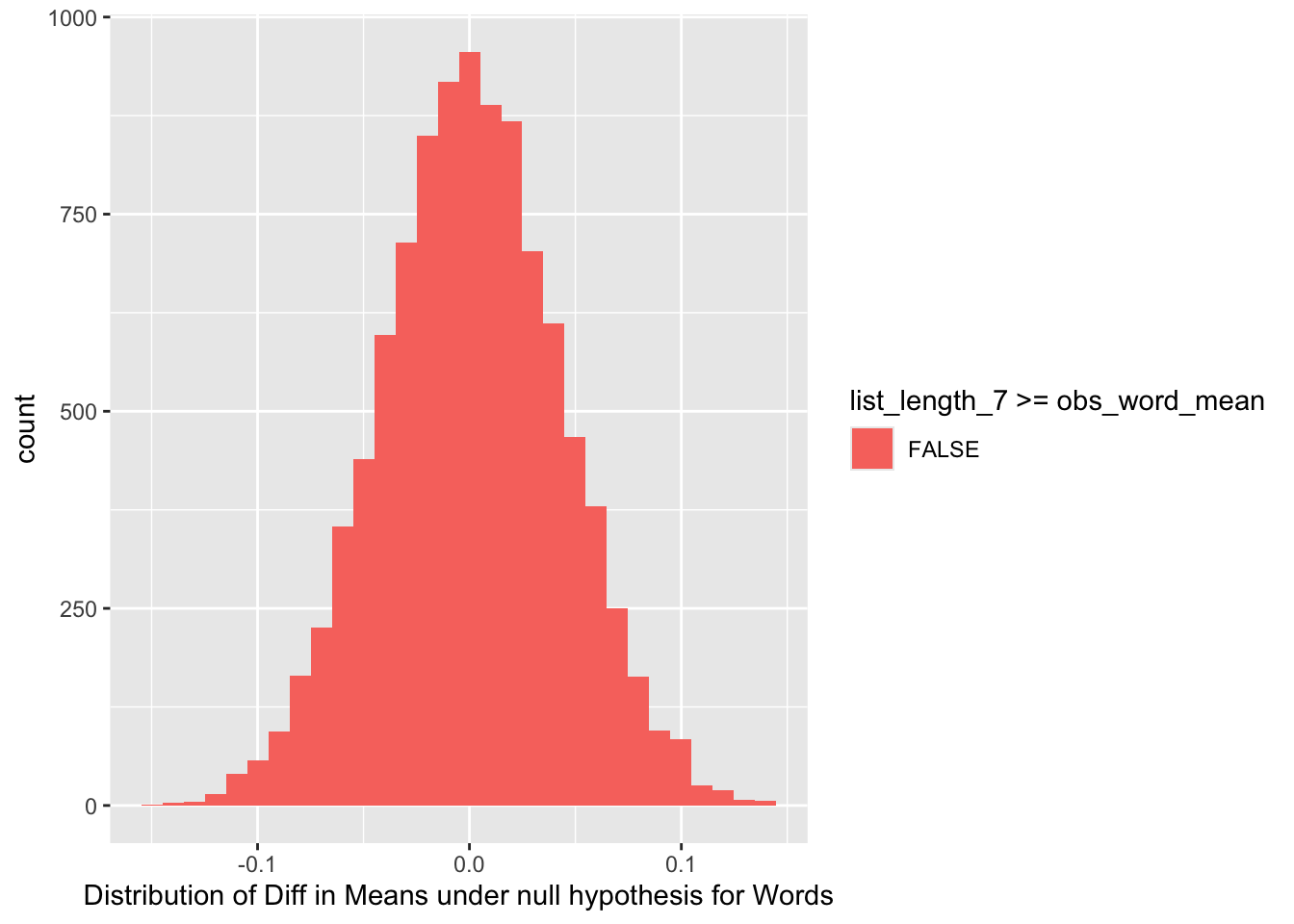
We proceed with a Permutation Test for each of the Parameters. We start with the Syllable Parameter SL. We shuffle the labels ( SL- = 2 and SL+ = 5) between the scores and determine the null distribution. This is then compared with the difference in mean scores between the unpermuted sets. We continue similarly for the other two parameters.
## [1] 0.0153731## syllable_5
## 1 0.007965635
## 2 0.002240714
## 3 0.040367063
## 4 0.005366587
## 5 0.011110556
## 6 0.025703095## [1] 0.08526183## study_time_30
## 1 -0.009797857
## 2 -0.074956746
## 3 -0.042852937
## 4 0.046689921
## 5 -0.006070397
## 6 -0.026399603## [1] 0.2887539## list_length_7
## 1 -0.07019373
## 2 0.03808659
## 3 -0.06223960
## 4 -0.03589373
## 5 0.04951119
## 6 -0.02442849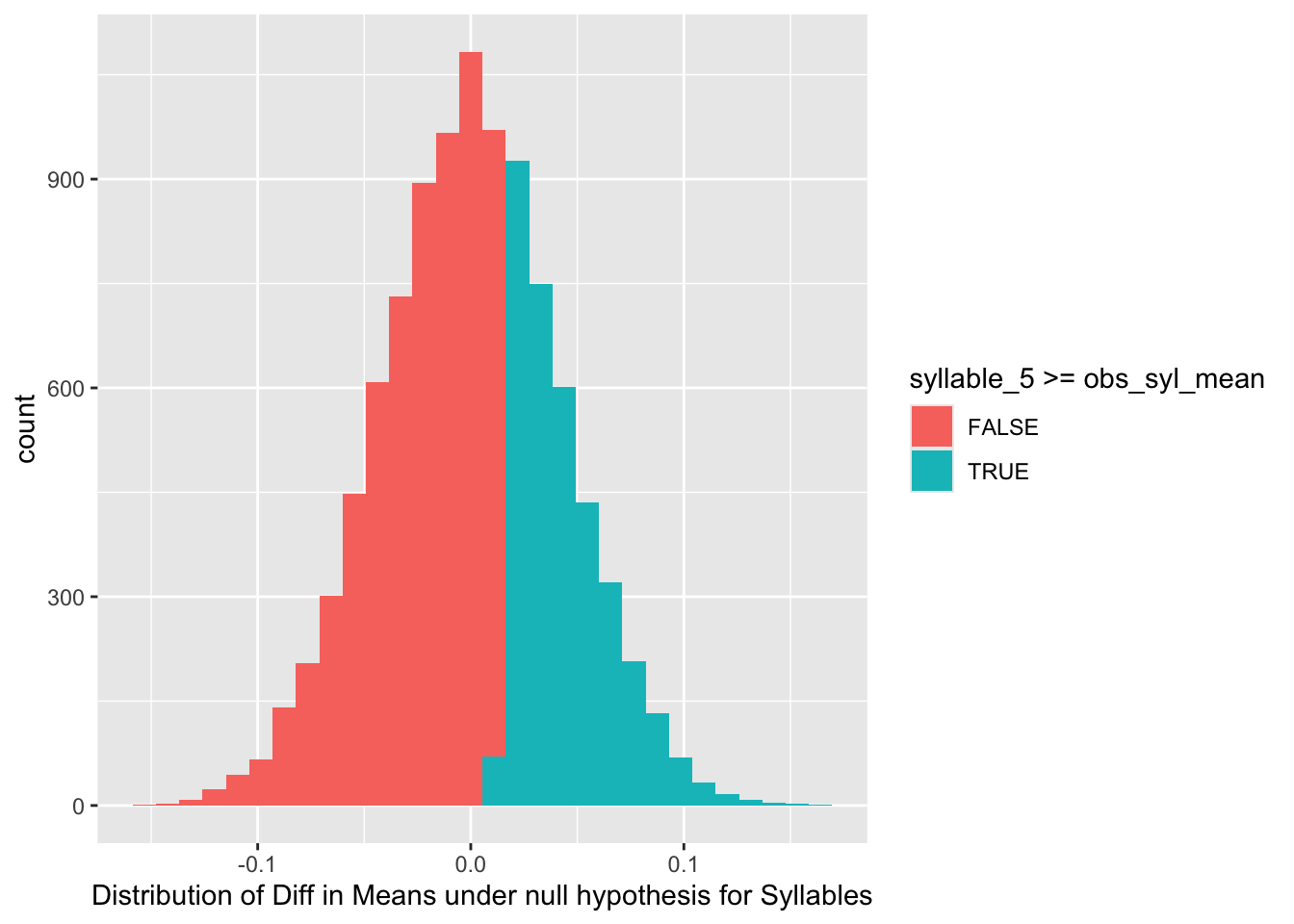
Conclusions
From the above null distribution plots obtained using Permutation tests, it is clear that both Study Time ( ST ) and List Word Length ( WL) have significant effects on the Short Term Memory Scores. The probability that the observed value is obtained or exceeded by any permutation of scores is very low in both cases.
On the other hand, Syllable Count (SL) does not seem to affect the STM scores significantly.
References
Lawrance, A. J. 1996. “A Design of Experiments Workshop as an Introduction to Statistics.” American Statistician 50 (2): 156–58. doi:10.1080/00031305.1996.10474364.↩︎
Ernst, Michael D. 2004. “Permutation Methods: A Basis for Exact Inference.” Statistical Science 19 (4): 676–85. doi:10.1214/088342304000000396.↩︎
Pruim R, Kaplan DT, Horton NJ (2017). “The mosaic Package: Helping Students to ‘Think with Data’ Using R.” The R Journal, 9(1), 77–102. https://journal.r-project.org/archive/2017/RJ-2017-024/index.html.↩︎