How does one read Shakespeare?
To code or not to code, that is the question...
gg is for Grammar of Graphics
Data
Aesthetics
Geoms
+ geom_*()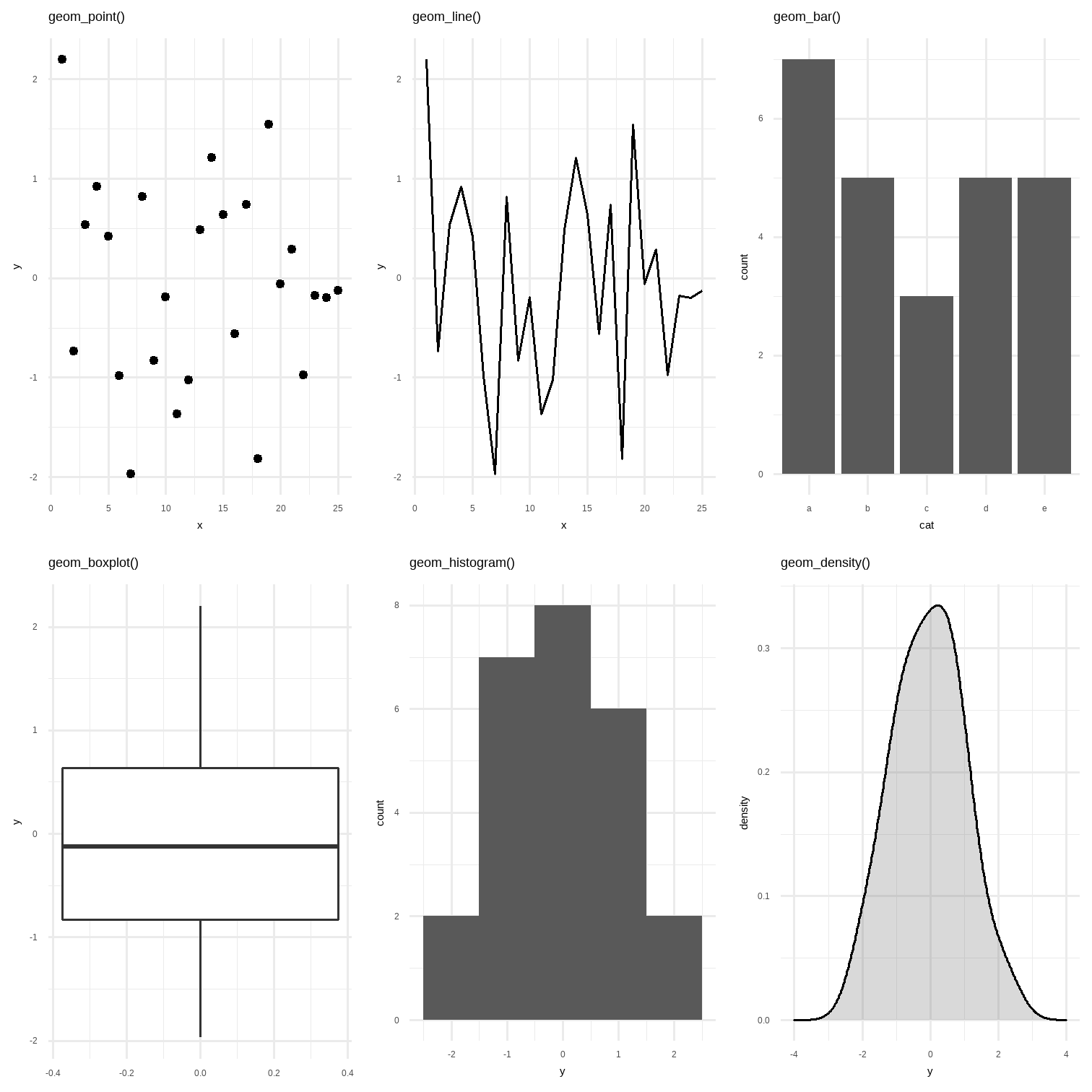
Chunk: Mapping
ggplot(penguins)
Chunk: Mapping
ggplot(data = penguins, mapping = aes(x = bill_length_mm, y = body_mass_g))
Chunk: Mapping
ggplot(data = penguins, mapping = aes(x = bill_length_mm, y = body_mass_g)) + geom_point()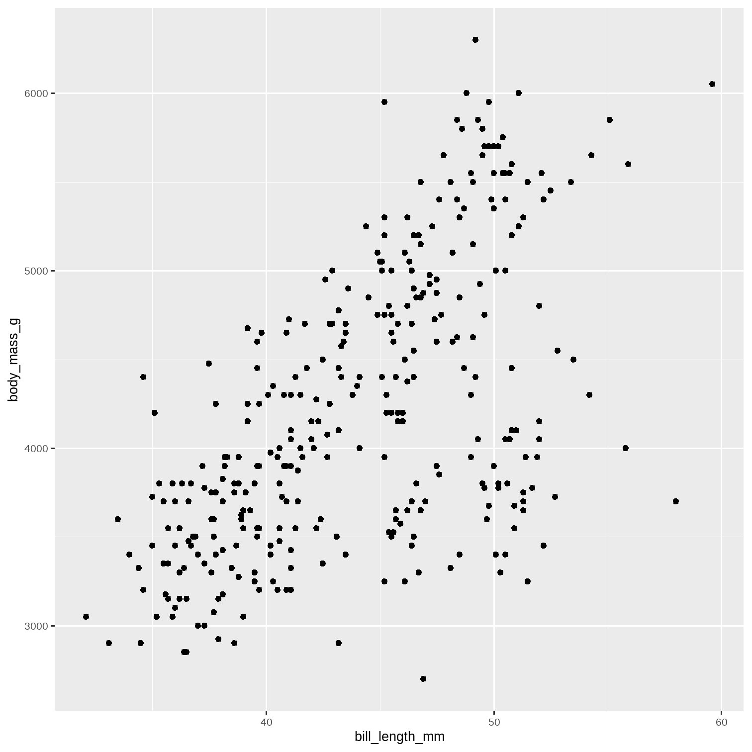
Chunk: Mapping
ggplot(data = penguins, mapping = aes(x = bill_length_mm, y = body_mass_g)) + geom_point() + geom_smooth(method = "lm")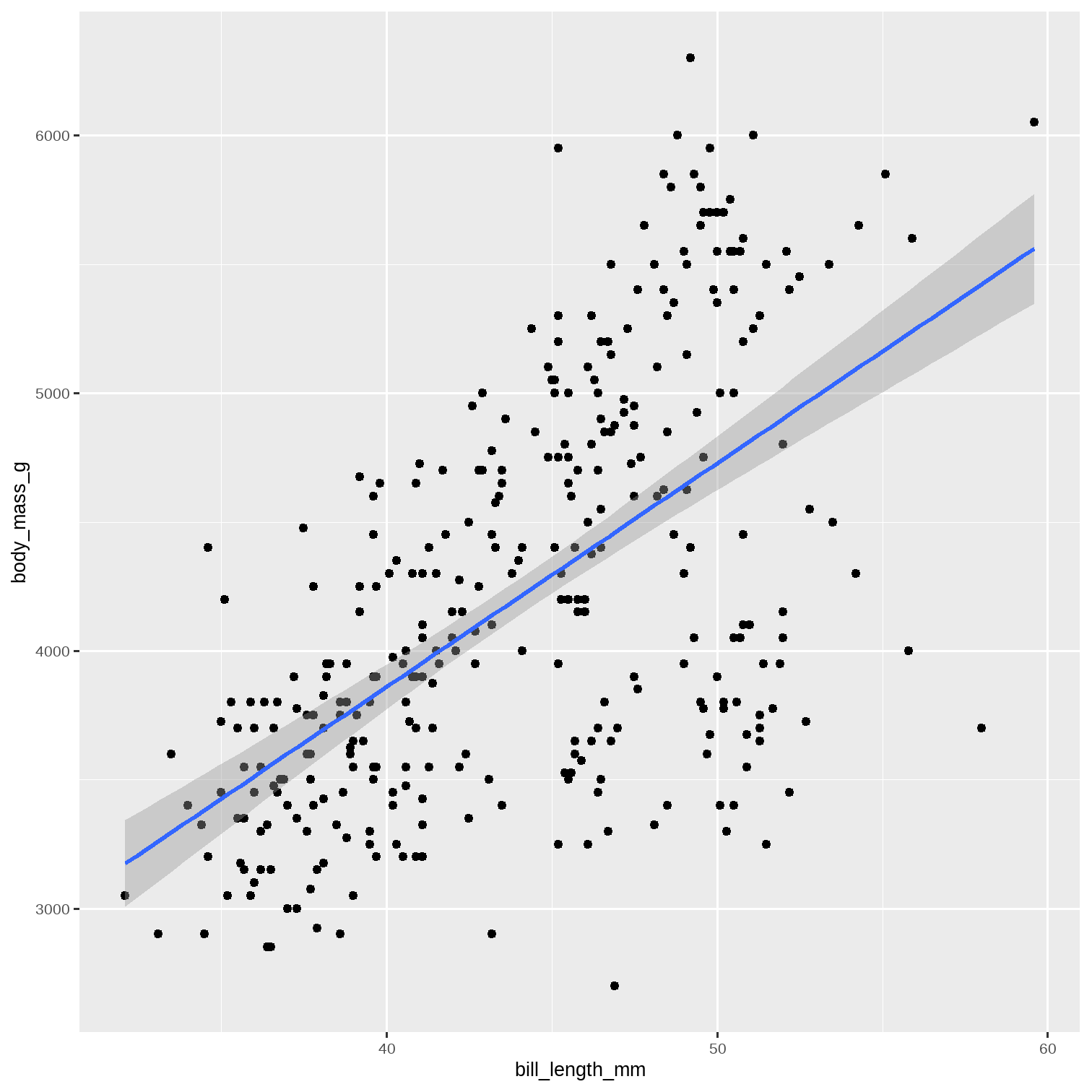
Chunk: Geom_Point_Position_Colour
ggplot(data = penguins)
Chunk: Geom_Point_Position_Colour
ggplot(data = penguins, aes(x = bill_length_mm, y = body_mass_g, color = island))We can leave out the "mapping" word and just use aes .
Why is there no plot?
🤔 💭
Right !! We have not used a geom command yet!!

Chunk: Geom_Point_Position_Colour
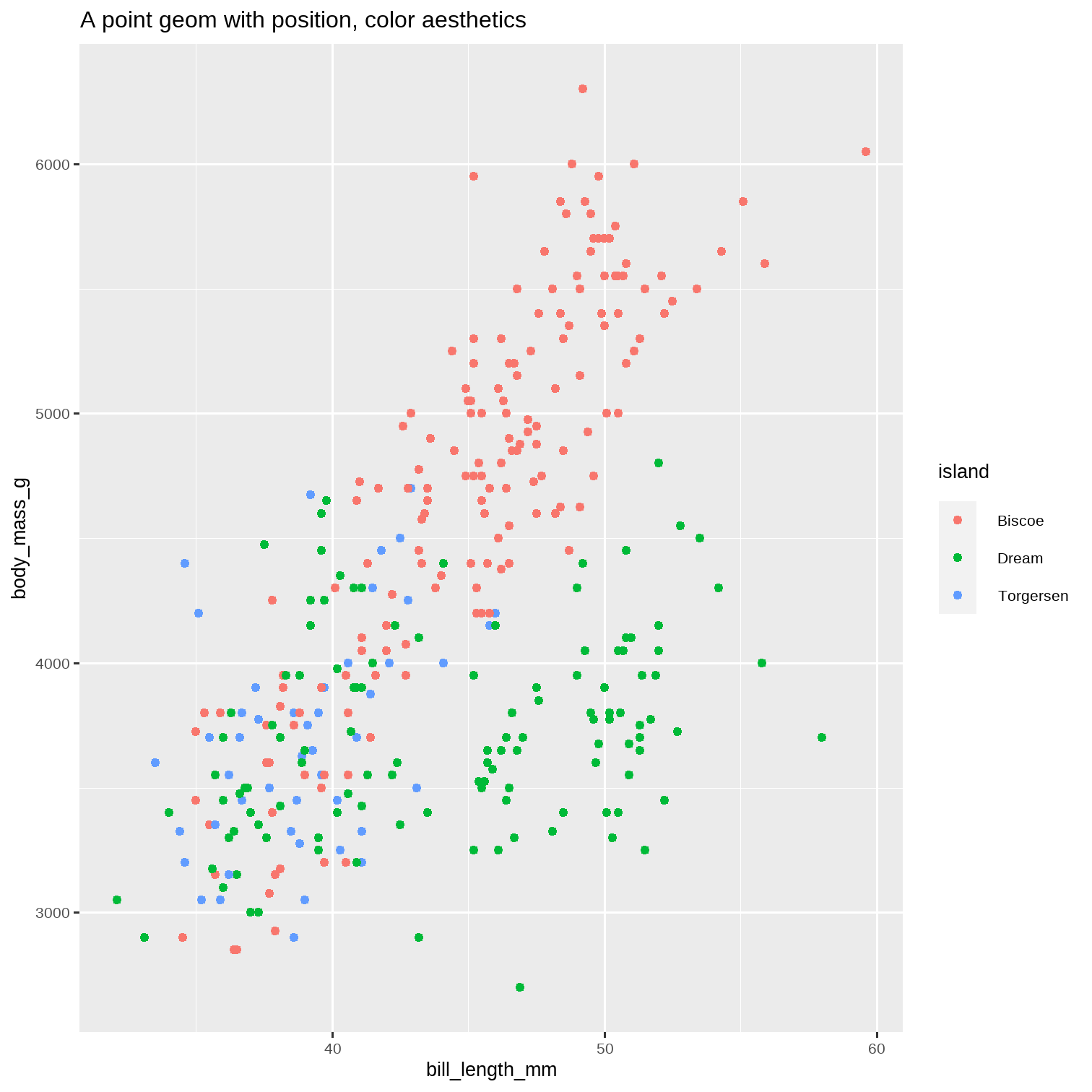
ggplot(data = penguins, aes(x = bill_length_mm, y = body_mass_g, color = island)) + geom_point() + ggtitle("A point geom with position, color aesthetics")Note that the points are located by position coordinates on both x and y axis, and coloured by the island variable.
Chunk: Geom_Point_Position_Colour
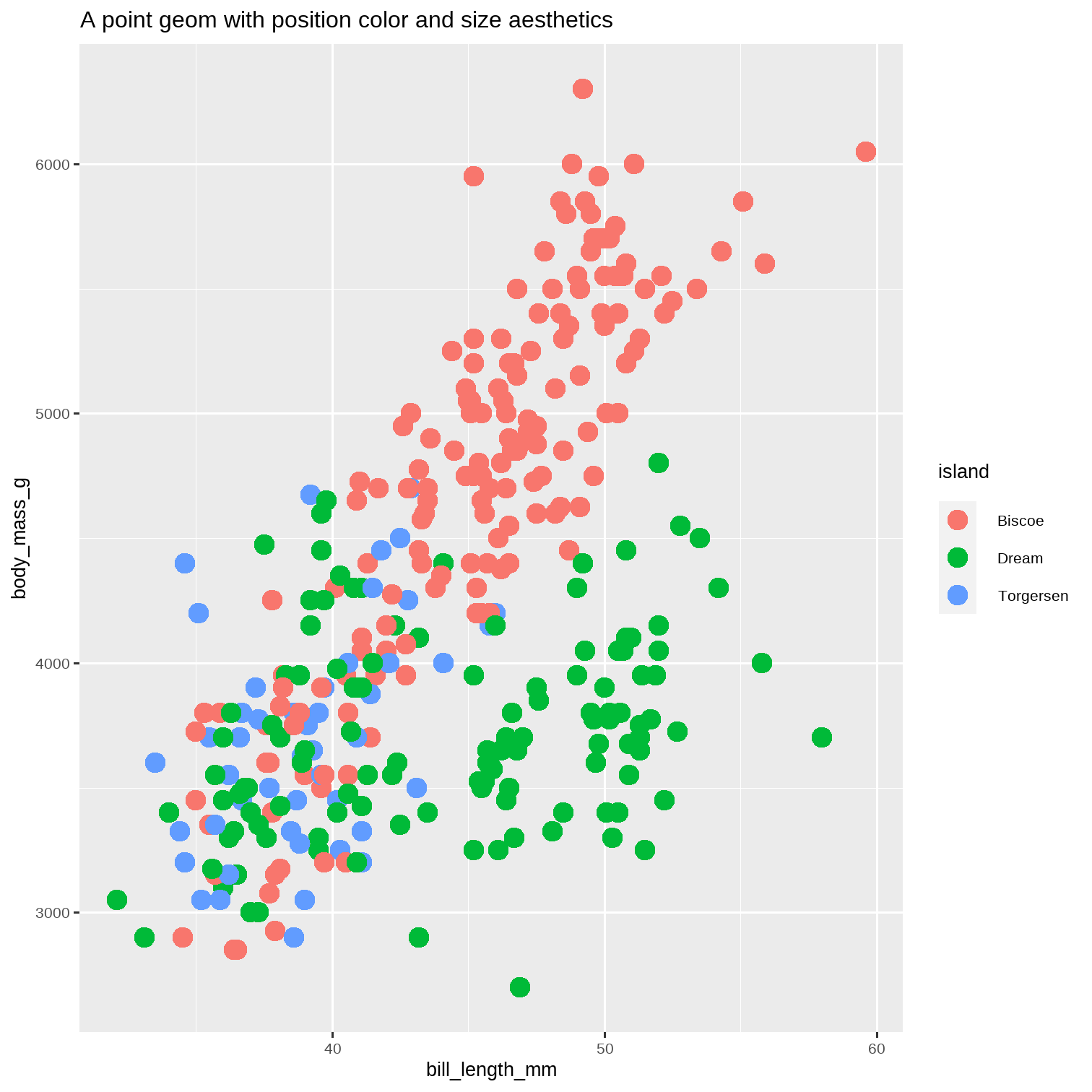
ggplot(data = penguins, aes(x = bill_length_mm, y = body_mass_g, color = island)) + geom_point(size = 4) + ggtitle("A point geom with position color and size aesthetics")Note that the points are located by position coordinates on both x and y axis, and coloured by the island variable.
And we've fixed size = 4!
Alpha
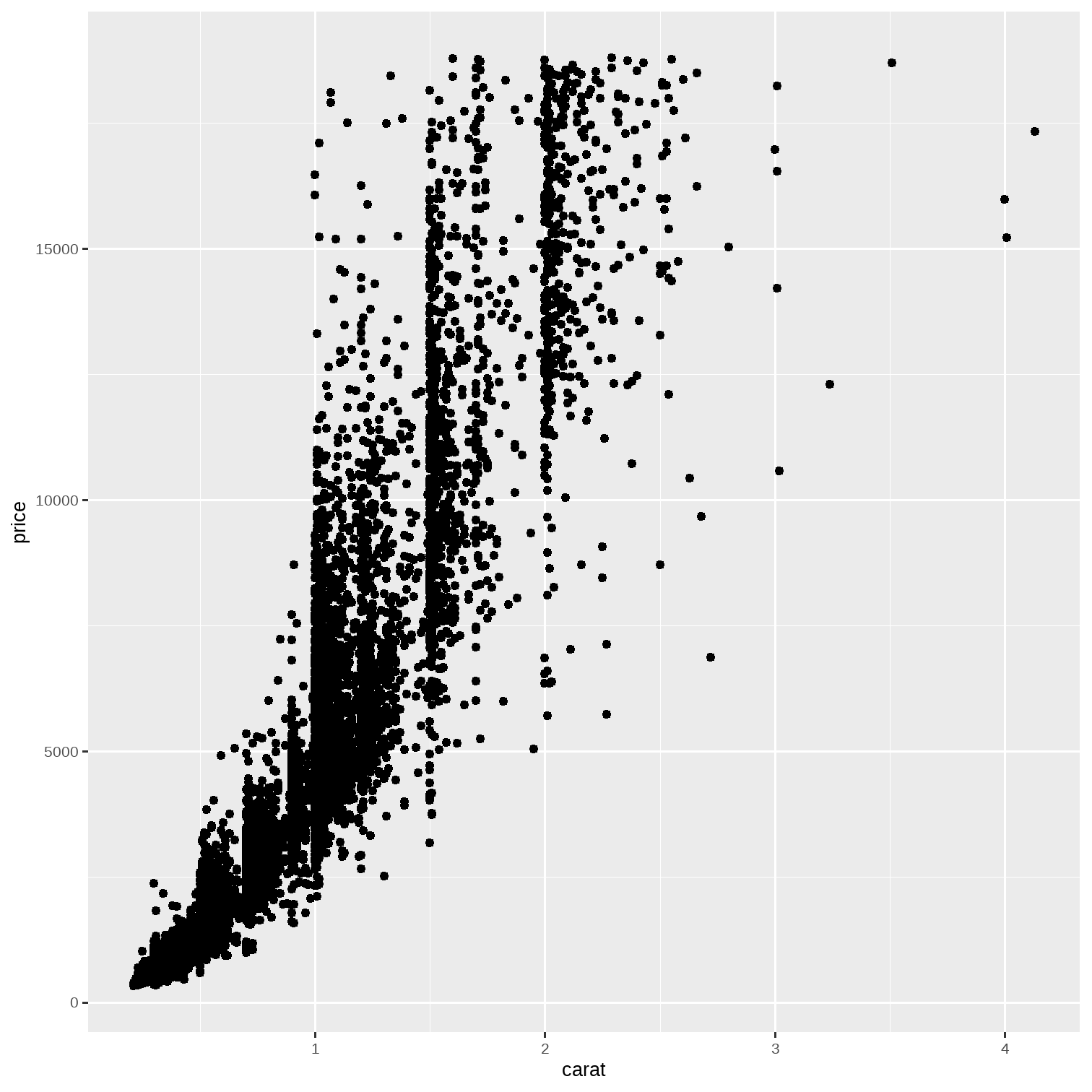
diamonds %>% # Sample some 20% of the data slice_sample(prop = 0.2) %>% ggplot(.) + geom_point(aes(x = carat, y = price))Are the points all overlapping? Can we see them better?
Alpha
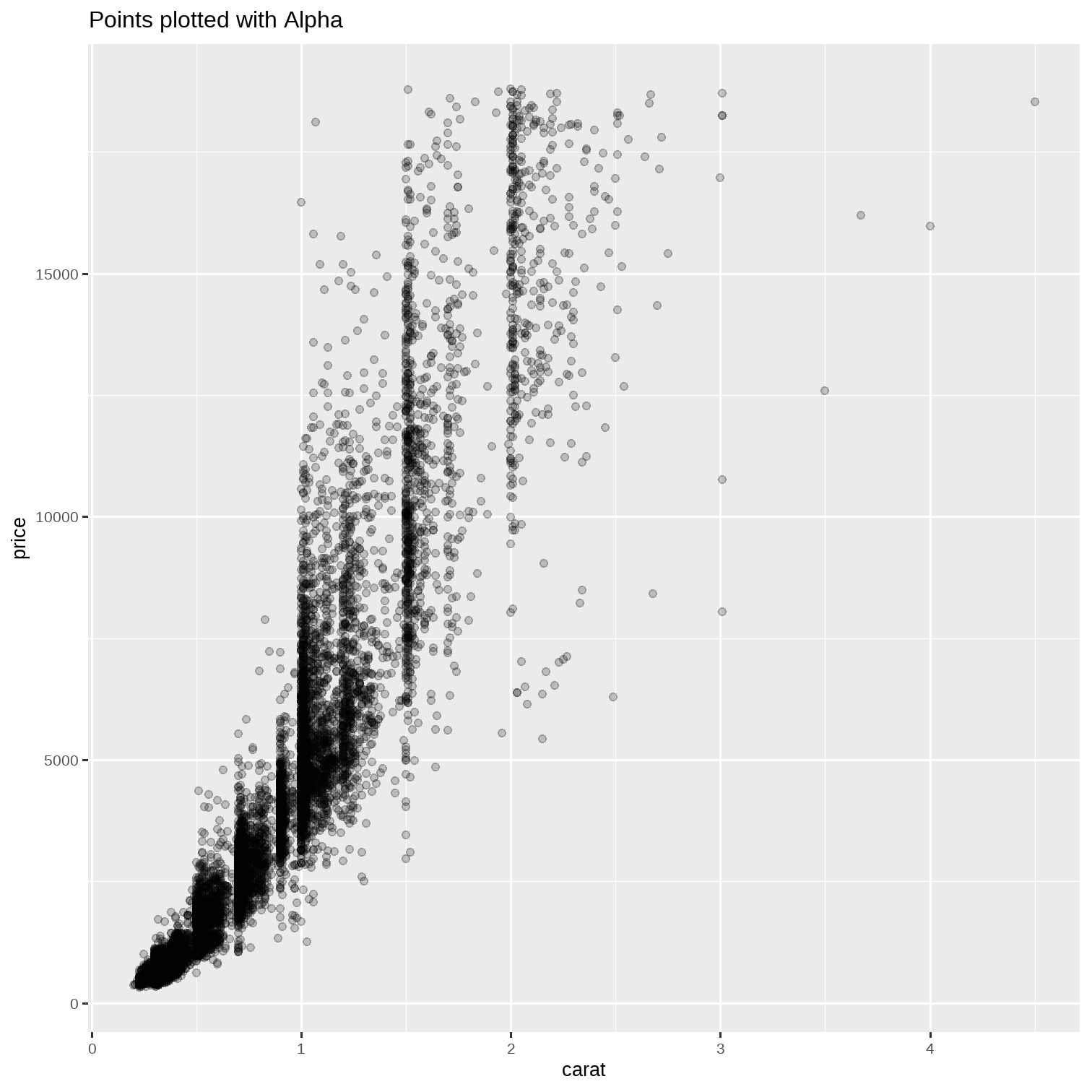
diamonds %>% # Sample some 20% of the data slice_sample(prop = 0.2) %>% ggplot(.) + geom_point(aes(x = carat, y = price), # alpha outside the aes() !!! alpha = 0.2) + labs(title = "Points plotted with Alpha")Are the points all overlapping? Can we see them better?
Chunk: Box Plot
ggplot(diamonds) + geom_boxplot(aes(x = cut, y = price)) + labs(title = "Box Plot")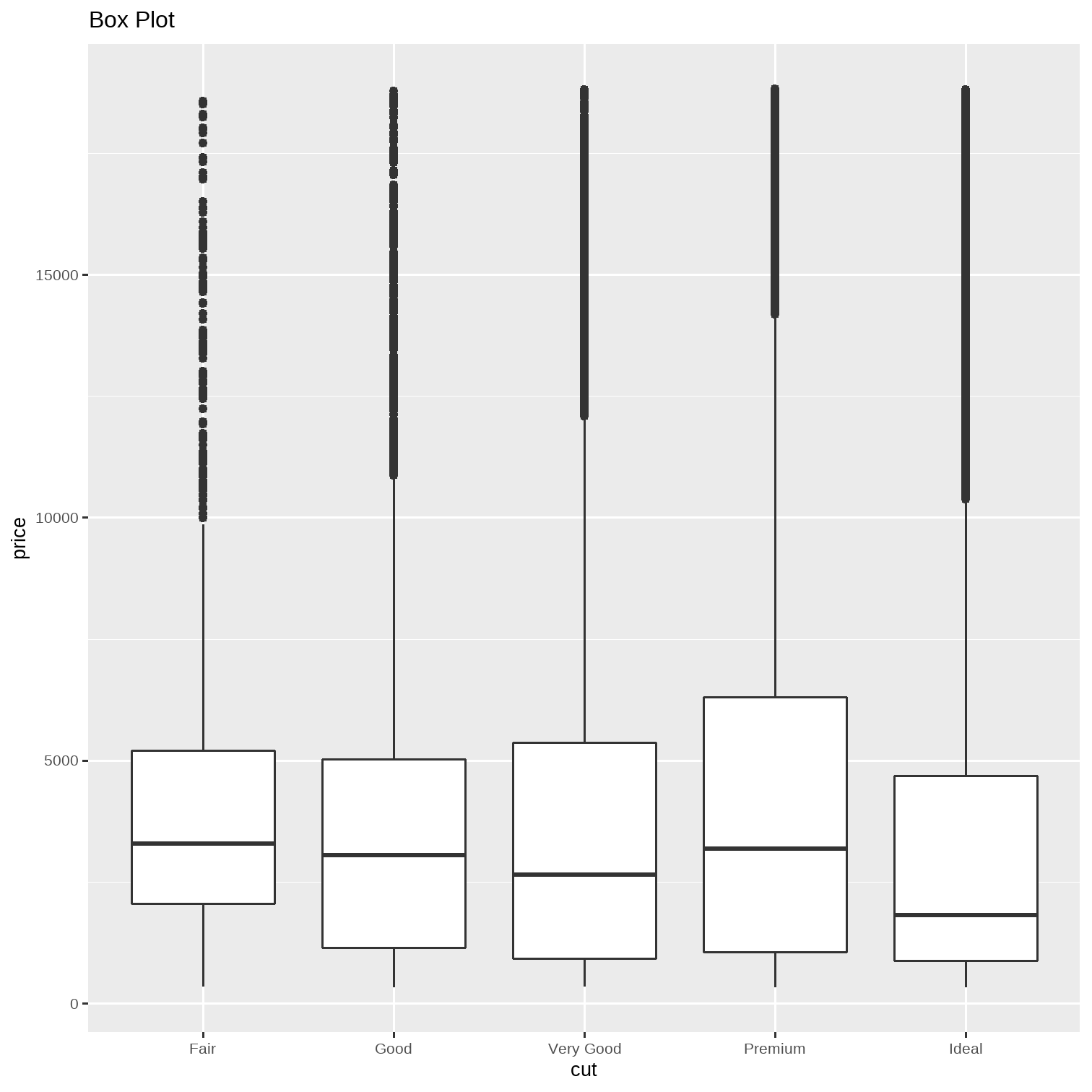
Chunk: Box Plot
ggplot(diamonds) + geom_boxplot(aes(x = cut, y = price, fill = cut)) + labs(title = "Box Plot")
Chunk: Geom_Bar_1
ggplot(data = penguins)
Chunk: Geom_Bar_1
ggplot(data = penguins) + aes(x = species)
Chunk: Geom_Bar_1
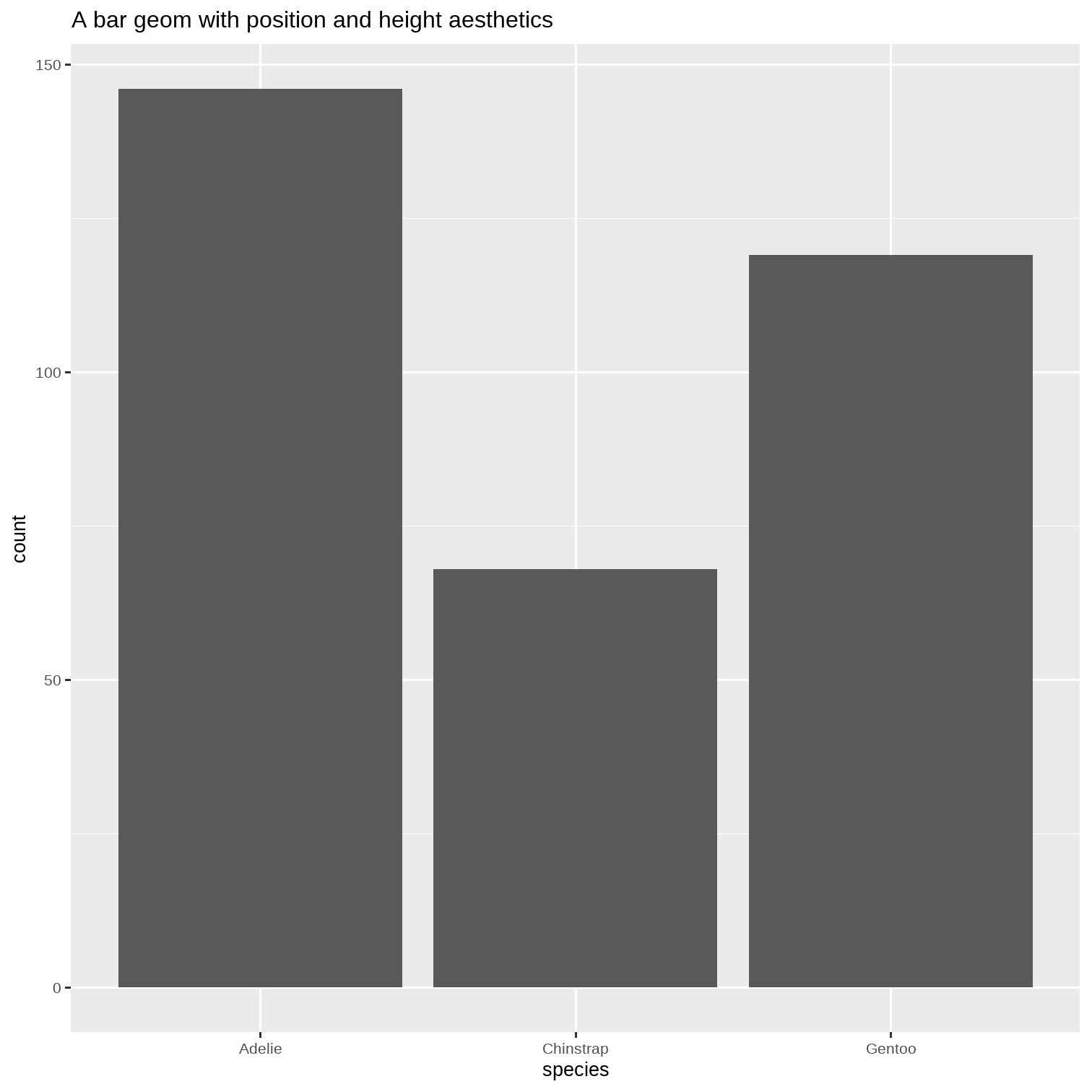
ggplot(data = penguins) + aes(x = species) + geom_bar() + ggtitle("A bar geom with position and height aesthetics")The bars are plotted with positions on the x-axis, defined by the species variable, and heights mapped to the y-axis.
How did the graph "know" the heights of the bars?
geom_bar has an internal count statistic computation.
Many geom_s have internal computation that are accessible to programmers.
Geom_Bar_Position_Stack_and_Dodge
When using more than a pair of variables with a bar chart, we have a few more position options:
ggplot(penguins, aes(x = species, fill = island))
Geom_Bar_Position_Stack_and_Dodge
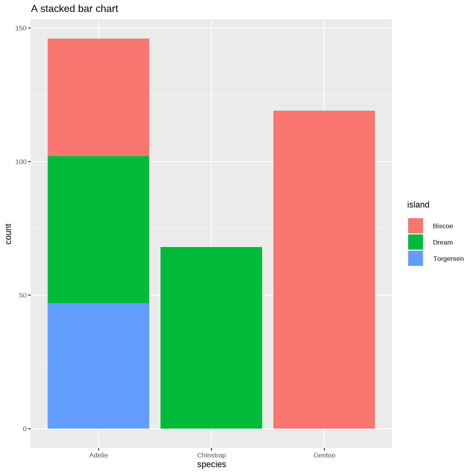
When using more than a pair of variables with a bar chart, we have a few more position options:
ggplot(penguins, aes(x = species, fill = island)) + geom_bar() + ggtitle(label = "A stacked bar chart")The bars are coloured by the island variable and are stacked in position.
Geom_Bar_Position_Stack_and_Dodge
And here we use the dodge option:
ggplot(penguins, aes(x = species, fill = island)) + geom_bar(position ="dodge") + ggtitle(label = "A dodged bar chart")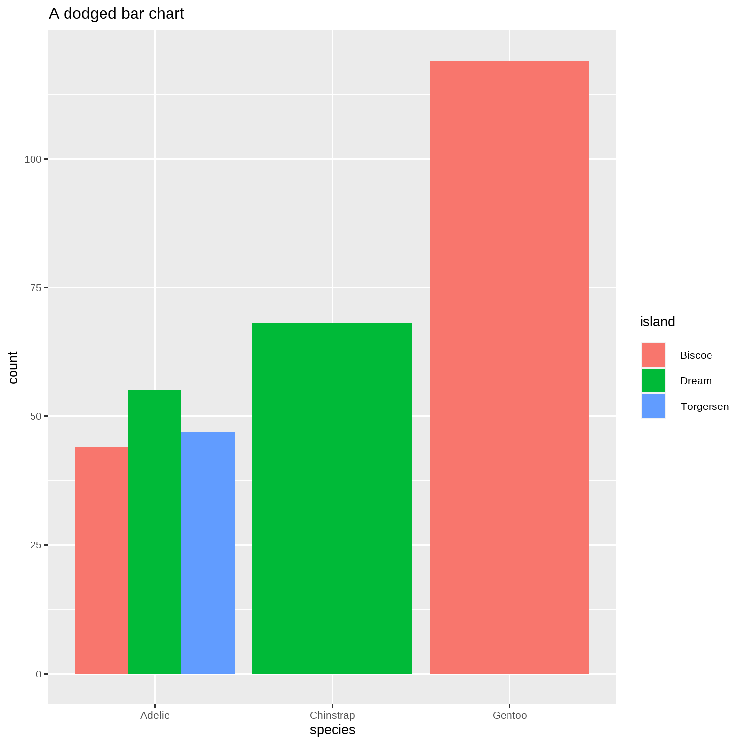
Facetting
ggplot(penguins)
Facetting
ggplot(penguins) + aes(x = flipper_length_mm, y = body_mass_g)
Facetting
ggplot(penguins) + aes(x = flipper_length_mm, y = body_mass_g) + geom_point()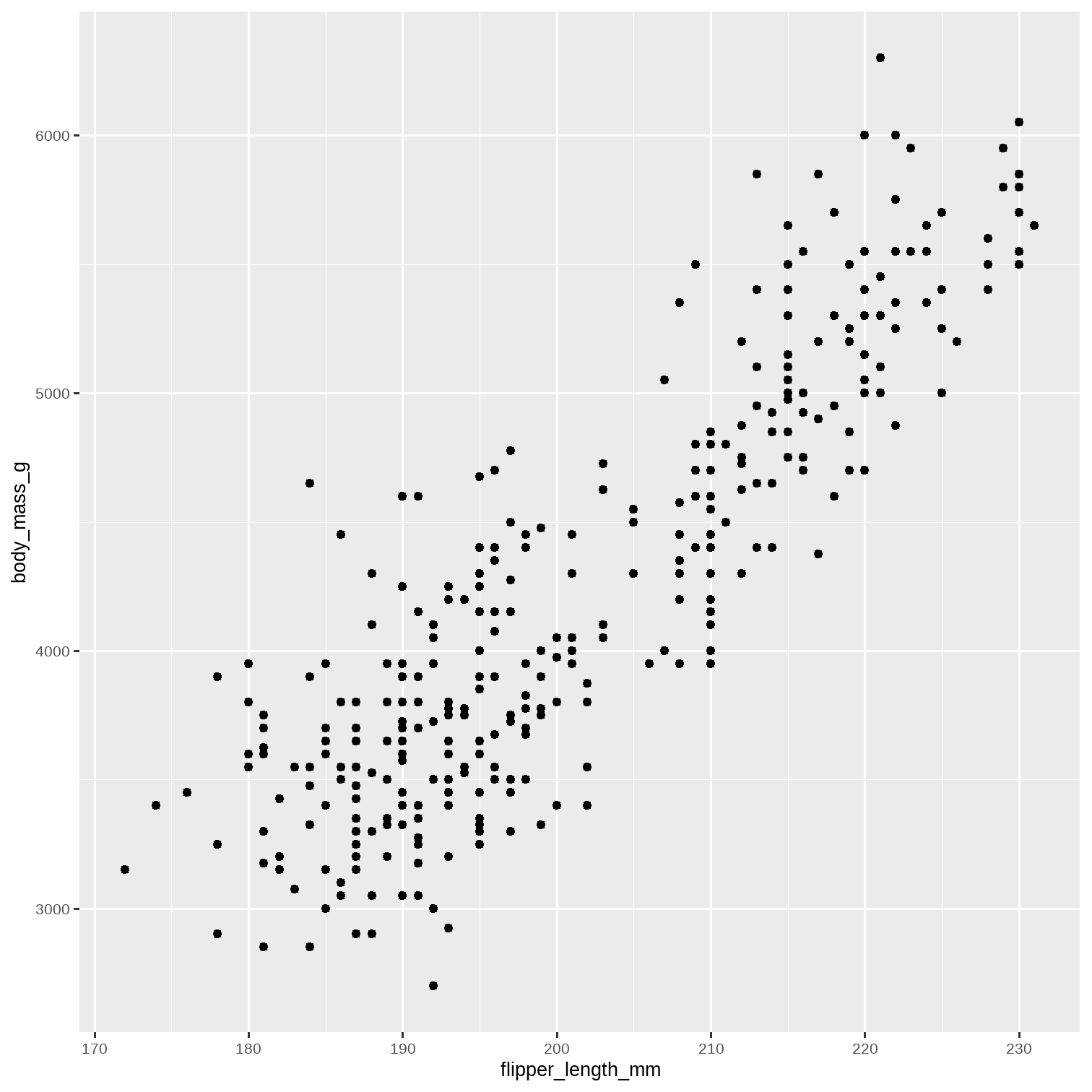
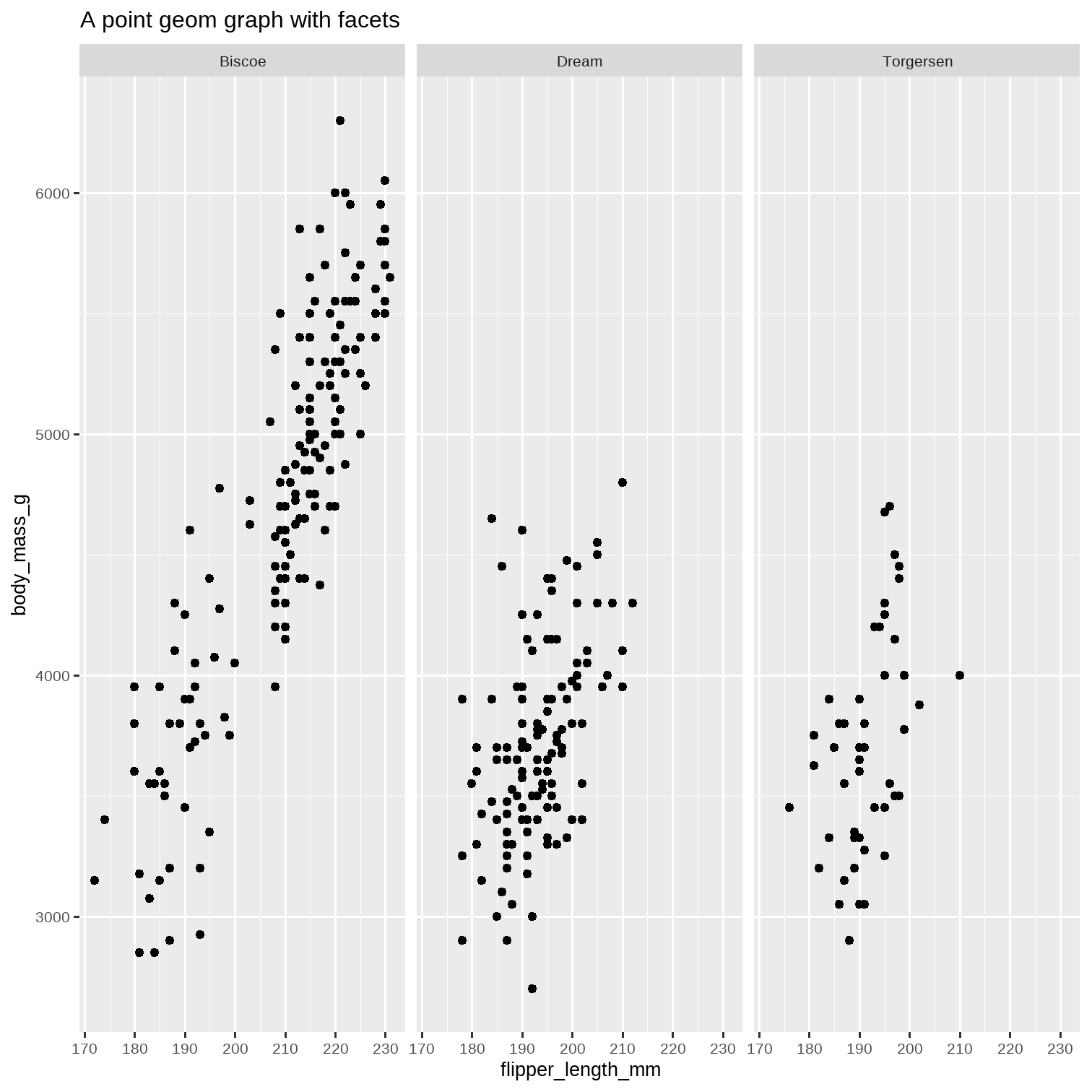
Facetting
ggplot(penguins) + aes(x = flipper_length_mm, y = body_mass_g) + geom_point() + facet_wrap(~island) + ggtitle("A point geom graph with facets")The graph has split into multiples, based on the number of islands.
Still more Facetting
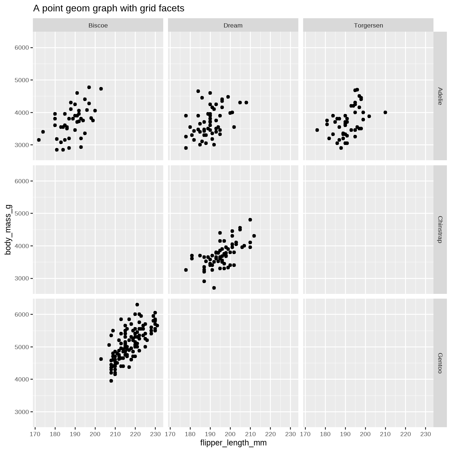
ggplot(penguins) + aes(x = flipper_length_mm, y = body_mass_g) + geom_point()What if we have even more "factor" variables?
We have island and species...can we split further?

Still more Facetting
ggplot(penguins) + aes(x = flipper_length_mm, y = body_mass_g) + geom_point() + facet_grid(species~island) + ggtitle("A point geom graph with grid facets")The graph has split into multiples, based on the number of islands and the number of species.
Finally...Colour !! ( Just a bit )
diamonds %>% slice_sample(prop = 0.2) %>% ggplot(.) + geom_point(aes(x = carat, y = price))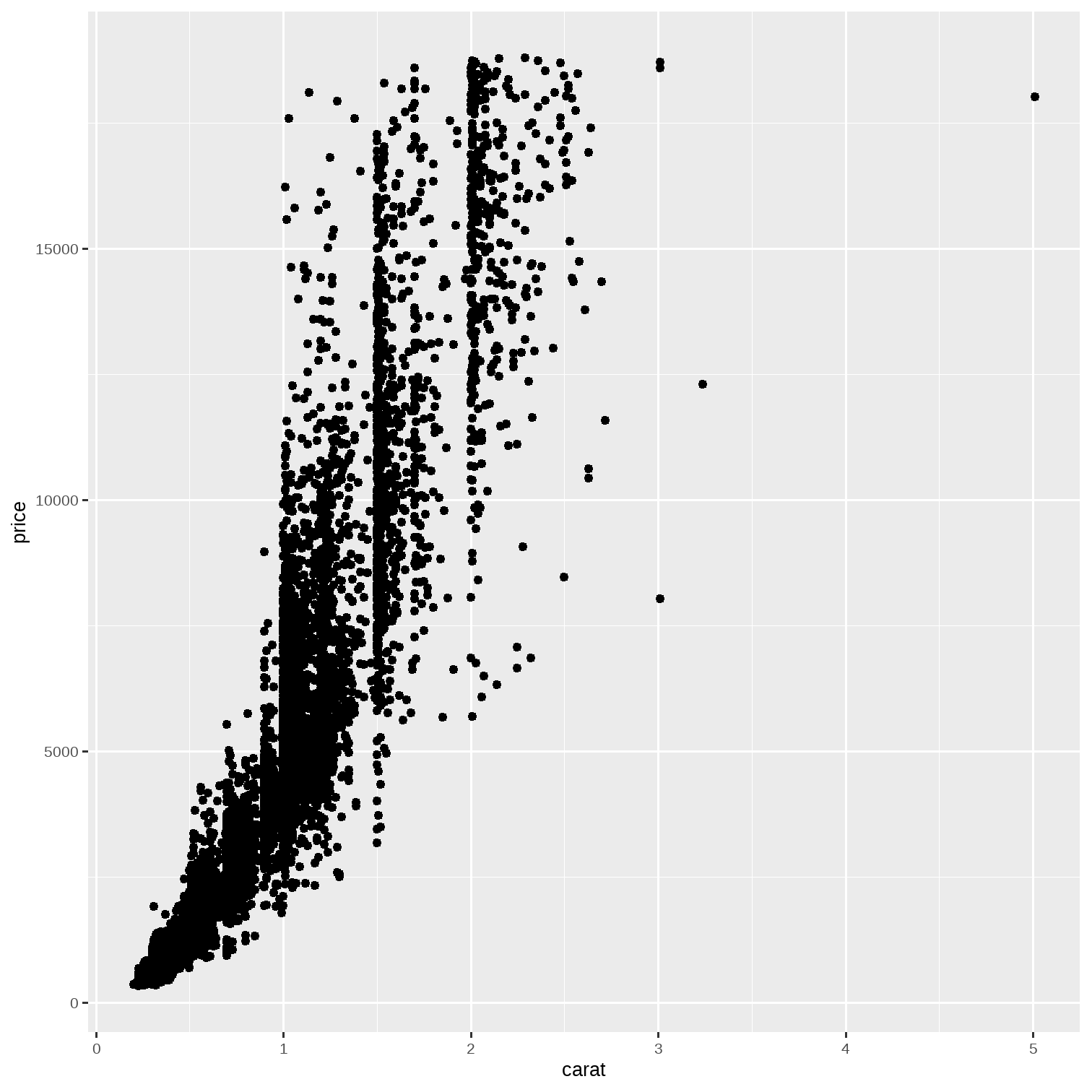
Finally...Colour !! ( Just a bit )
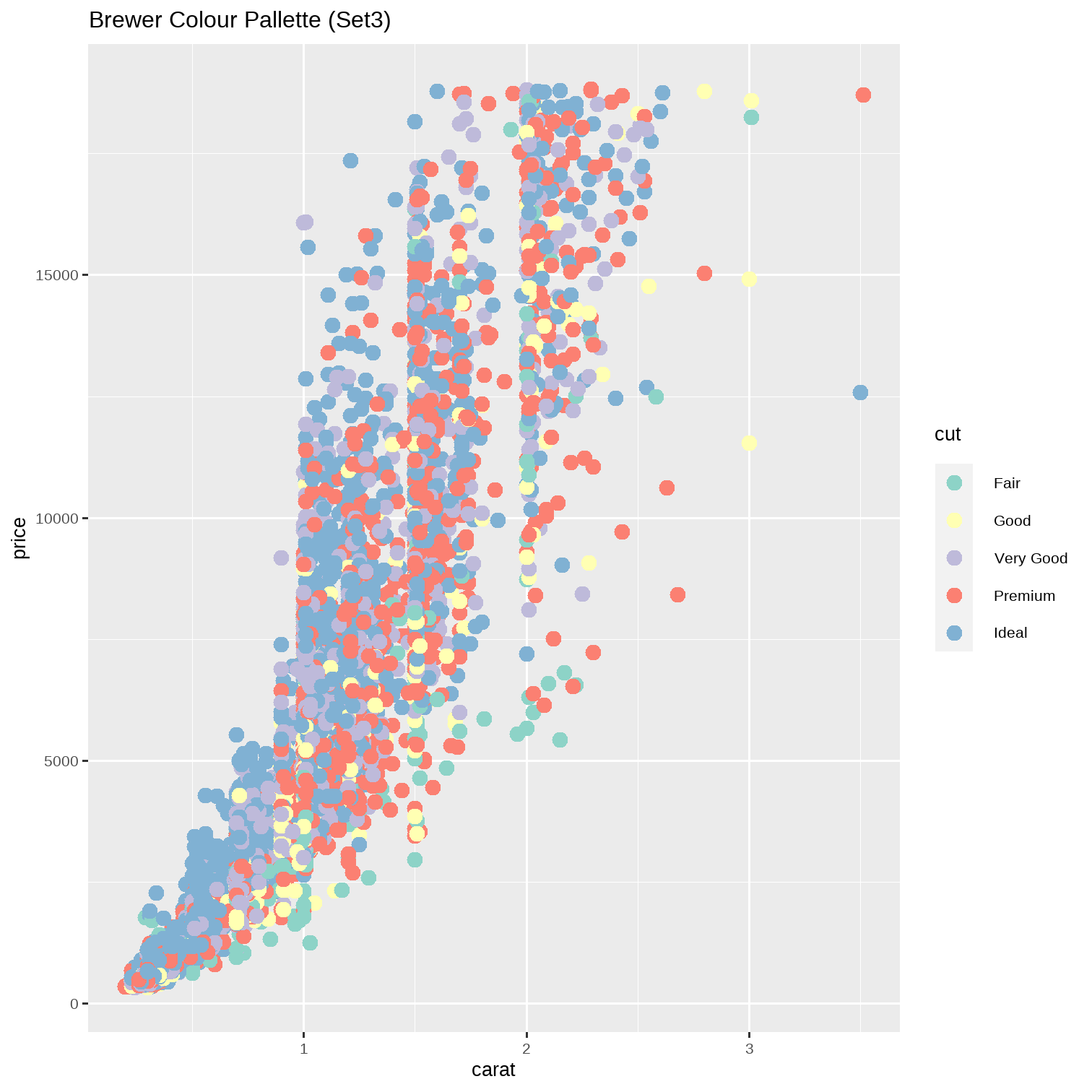
diamonds %>% slice_sample(prop = 0.2) %>% ggplot(.) + geom_point(aes(x = carat, y = price, colour = cut), size = 3) + scale_colour_brewer(palette = "Set3") + labs(title = "Brewer Colour Pallette (Set3)")We are using the RColorBrewer package here.
Type RColorBrewer::display.brewer.all() in your Console and see what palettes are available.
Chunk: Colour !! ( Just a bit )
diamonds %>% slice_sample(prop = 0.2) %>% ggplot(.) + geom_point(aes(x = carat, y = price, colour = cut), size = 3) + scale_colour_viridis_d() + labs(title = "Viridis Palette", subtitle = "The Default in ggplot")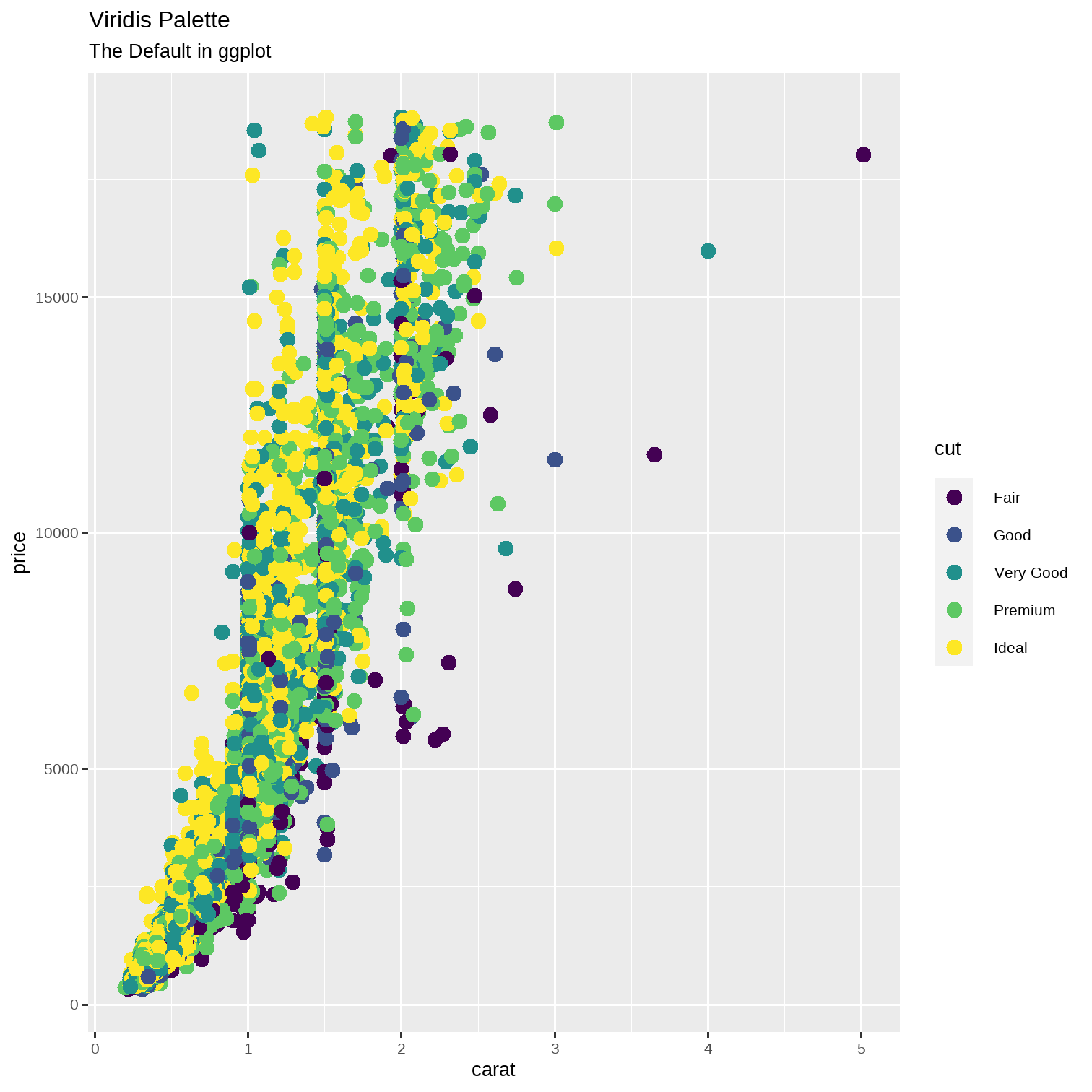
Chunk: Colour !! ( Just a bit )
diamonds %>% slice_sample(prop = 0.2) %>% ggplot(.) + geom_point(aes(x = carat, y = price, colour = cut), size = 3) + scale_colour_viridis_d(option = "magma") + labs(title = "Viridis Palette, Option Magma")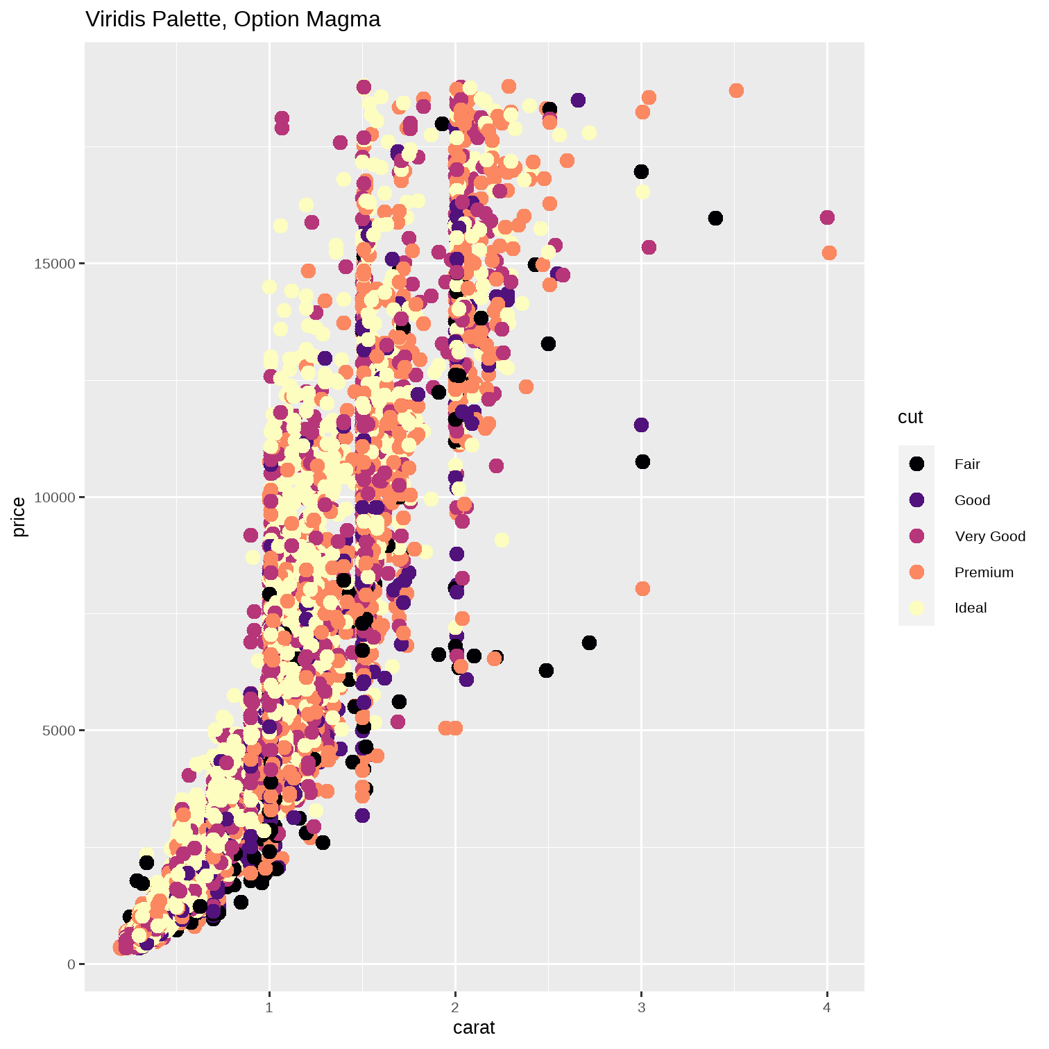
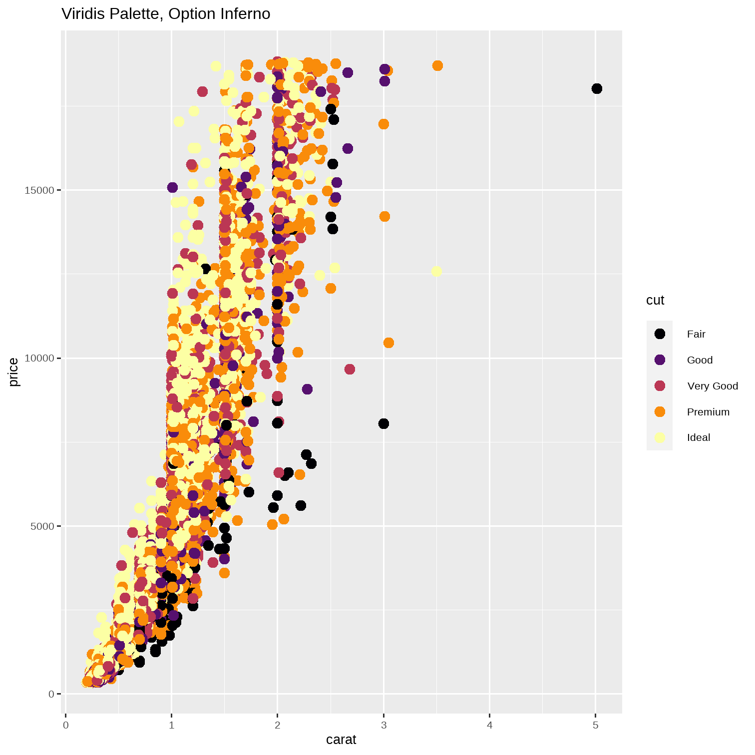
Chunk: Colour !! ( Just a bit )
diamonds %>% slice_sample(prop = 0.2) %>% ggplot(.) + geom_point(aes(x = carat, y = price, colour = cut), size = 3) + scale_colour_viridis_d(option = "inferno") + labs(title = "Viridis Palette, Option Inferno")