Eating Mangoes with Hamlet
 Tom und Nicki Löschner on Pixabay
Seeing Data
- Let us first examine the street traffic data we have gathered for any “model-like” pattern!
We will use a tool called, umm….WTFcsv. Let us first quickly see what this tool offers us!
Let us import our data into the WTFcsv tool (Web Link) and see what patterns lurk beneath our data!
- Let us throw some chalk or Lego pieces on the floor at random and see what happens!!
Is Randomness a Design Tool, then?

- Do you remember plucking mangoes from the trees in your childhood
gardens?
- Did you happen to be the youngest in the group?
- Did you have run home to get the salt + chilly powder?
- Why did you trust your friends not to eat off the best mangoes in your absence? ;-D
- Were you used to being the “denner” in every game?
- Was that a completely “mad” thing to do, throwing stuff on the floor? Or was it an act of Pedagogical Vandalism?
- Is Randomness just too much to handle or comprehend?
- Or can we “tame” it in some way, and put it to use in Art, Design, and Tech?
- Have we been doing this all along? Have we been “holding infinity in the palm of our hands”1, in the हाथ कीे लकीरे?
- What diagrams or thought experiments can we create to do this?
- WHY would this be a good idea? Is there a very Human Motivation behind this desire we might have?
Could this song indicate what our situation might be?
https://www.youtube.com/watch?v=qan0Y9hXpPQ
https://www.filmyquotes.com/songs/1381
Well, perhaps not entirely ;-D
Hamlet is also like us !!
Let us read the famous nunnery scene from Hamlet:
Hamlet in 4 Minutes:
To be or Not to be: (Web Link)
What was Hamlet’s problem? How did he solve that problem?
Suppose we were Hamlet….
What would we want to know?
- Who is our friend?
- What is the chance that we will survive?
- Who killed Dad?
Did Hamlet have an idea, any suspicion, that he might have wanted to prove? Yes, he did, and that is why he feigned madness, so people would open up and tell him things, in an unguarded way. So there was craft in his madness.
If we wanted to know the truth of something, some guess, or a Hypothesis that we had, then we would need to conduct an “Experiment”, rather like Hamlet did, without quite going or feigning madness of course. But there is a Madness to the Method, as we will see…

From StatsRef :
The PPDAC summary table suggests a relatively linear flow from problem definition/Hypothesis through to conclusions — this is typically not the case. It is often better to see the process as cyclical, with a series of feedback loops. A summary of a revised PPDAC approach is shown in the diagram below. As can be seen, although the clockwise sequence (1→5) applies as the principal flow, each stage may and often will feed back to the previous stage.
In addition, it may well be beneficial to examine the process in the reverse direction, starting with Problem definition and then examining expectations as to the format and structure of the Conclusions (without pre-judging the outcomes!). This procedure then continues, step-by-step, in an anti-clockwise manner (e→a) determining the implications of these expectations for each stage of the process.
Design of Experiments
Let us pretend we are Hamlet and design a simple experiment to find out some “truth” (highly probable idea) that is important to us.
For example:
Let us consider the Short Term Memory(STM) of Foundation Students; Or , we could use the Guilford Divergent Thinking Test for Alternative Uses as our vehicle for testing similar Hypotheses:
- STM scores are significantly different between students of Design and those of Art (;-O)
- Any other factors, not related to types of individuals, but more
like parameters of STM itself, such as:
- Word complexity (Syllables per Word)
- No of Words
- Exposure Time and Recall Time
- Students who speak their Mother Tongue fluently score better in Divergent Thinking Scores (Fluency, Flexibility, Elaboration, Originality)
- There is a significant difference in Guilford Scores between students from “small towns” and those from metros.
Factors
In each of these Hypotheses, we can see that there are binary
(two-valued) parameters that are part of the test: Art vs Design,
Speaks Mother Tongue or Not, Small Town vs Metro,
Long vs Short List of Words, Short vs Long Words and
Long vs Short Exposure.
If we want our experiment to be fair we must have:
Devise a test tool for each combination of binary parameters (Test Type)
the same number of subjects for each Test Type
randomly select the people as respondents each Test Type
We will choose one of these questions, or a similar one, and use the PPDAC Method to proceed with our Experiment. This paper by Lawrence to guide our Hypothesis Testing and the Design of our Experiment: Lawrence - A Design of Experiments Workshop as an Introduction to Statistics (Weblink to PDF). This is the paper describing a simple Design of Experiments workshop in class much like ours. We will try to mimic as much of this as we can. Do read through this in the evening today in preparation for our experiment.
Data Analysis-1: Comparison of STM Histograms using Excel and WTFcsv
Once our test is complete, let us collate all the data for all tests using Excel. (This is for the STM Hypothesis; we can adapt this spreadsheet for any other hypothesis test with categorical factors and scores.)
- Download this spreadsheet and save as your own named local copy.
- Enter the data from all tests on the first sheet titled “RawData” (the one with the warning)
- Duplicate this data on the sheet titled “Data Duplicated”. Do not touch the “RawData” sheet again.
- For each of the factors under consideration, we will need to stack
up STM scores from
- If we have three two-valued, categorical factors, we will get three sets of stacked scores, each from a (shuffled) set of the tests.
- Half the scores in these stacked columns will pertain to one level of the factor, and the other half of the scores will pertain to the other level. (This should remind you of the Karnaugh Map you may have learnt in your digital logic courses in school.). See example below: it shows how we can stack up the scores from 4 tests for each level of the parameter p1.
##   scores test    p1    p2    p3
## 1     20    A  True  Long   Big
## 2     20    B  True  Long Small
## 3     20    C  True Short   Big
## 4     20    D  True Short Small
## 5     20    E False  Long   Big
## 6     20    F False  Long Small
## 7     20    G False Short   Big
## 8     20    H False Short Small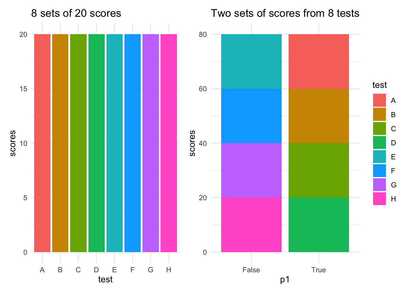
- We will set up each of these two stacked-score columns in Col A on separate sheets, similar to the one shown in the sheet titled “Permutation Test”. One sheet for each two-valued parameter.
- Create paired Histograms for each of the two stacked-score columns using WTFcsv, or Excel itself if you are confident. Ensure that there are TWO Histograms: one for each value of the factor under consideration.
- Inspection of the shapes and locations of these paired Histograms may give you an idea whether the factor under consideration has any effect on STM scores or none.
## Warning: Using `size` aesthetic for lines was deprecated in ggplot2 3.4.0.
## ℹ Please use `linewidth` instead.
## This warning is displayed once every 8 hours.
## Call `lifecycle::last_lifecycle_warnings()` to see where this warning was
## generated.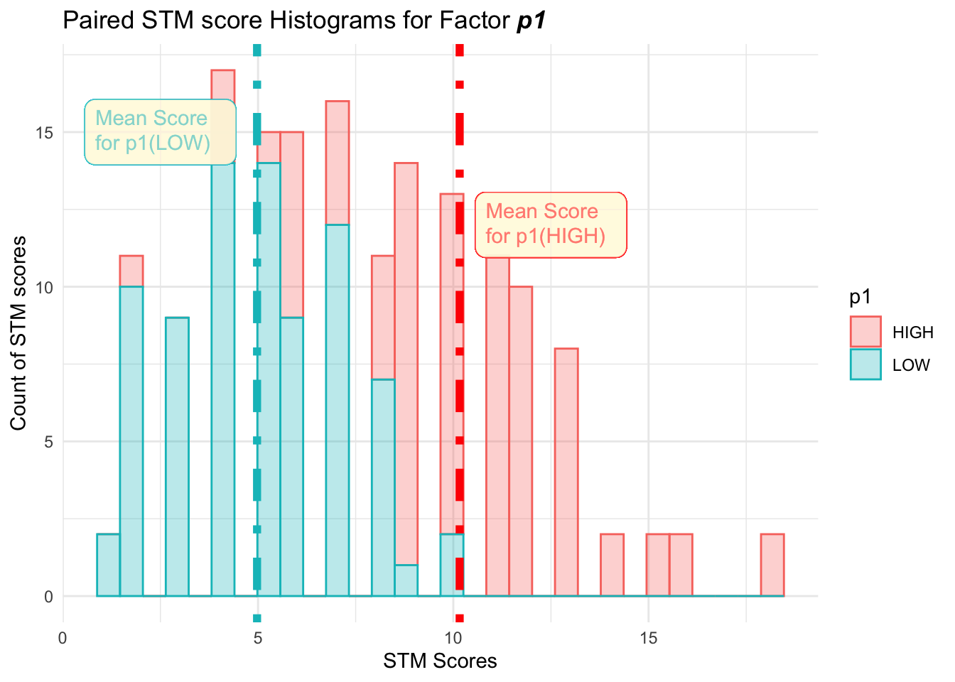
- Save these 6 histograms as PNG files on your machines and use them along with Comic Generator (discussed below) to tell the story of your Hypothesis Testing.
Computing Parallel Worlds: The Permutation Test
What is we cannot trust our eyes to compare the pair-wise Histograms?
If there was considerable overlap?
Is there a better way? Yes by playing another Childhood Game, with a deck of cards !!!
Before we play with cards, some background
From: Tim C. Hesterberg (2015) What Teachers Should Know About the Bootstrap: Resampling in the Undergraduate Statistics Curriculum, The American Statistician, 69:4, 371-386, DOI: 10.1080/00031305.2015.1089789
Student B. R. was annoyed by TV commercials. He suspected that there were more commercials in the “basic” TV channels, the ones that come with a cable TV subscription, than in the “extended” channels you pay extra for. To check this, he collected the data shown in Table 1. He measured an average of 9.21 minutes of commercials per half hour in the basic channels, vs only 6.87 minutes in the extended channels. This seems to support his hypothesis. But there is not much data—perhaps the difference was just random. The poor guy could only stand to watch 20 random half hours of TV. Actually, he didn’t even do that—he got his girlfriend to watch half of it. (Are you as appalled by the deluge of commercials as I am? This is per half-hour!)
| basic | extended |
|---|---|
| 6.950 | 3.383 |
| 10.013 | 7.800 |
| 10.620 | 9.416 |
| 10.150 | 4.660 |
| 8.583 | 5.360 |
| 7.620 | 7.630 |
| 8.233 | 4.950 |
| 10.350 | 8.013 |
| 11.016 | 7.800 |
| 8.516 | 9.580 |
## [1] 2.3459The average difference in ad times between the two sets of TV channels is 2.34.
How easy would it be for a difference of 2.34 minutes to occur just by chance? To answer this, we suppose there really is no difference between the two groups, that “basic” and “extended” are just labels. So what would happen if we assign labels randomly? How often would a difference like 2.34 occur?
We’ll pool all twenty observations, randomly pick 10 of them to label “basic” and label the rest “extended”, and compute the difference in means between the two groups. We’ll repeat that many times, say ten thousand, to get the permutation distribution shown in Figure 1.
| channel | times |
|---|---|
| basic | 6.950 |
| extended | 3.383 |
| basic | 10.013 |
| extended | 7.800 |
| basic | 10.620 |
| extended | 9.416 |
| basic | 10.150 |
| extended | 4.660 |
| basic | 8.583 |
| extended | 5.360 |
| basic | 7.620 |
| extended | 7.630 |
| basic | 8.233 |
| extended | 4.950 |
| basic | 10.350 |
| extended | 8.013 |
| basic | 11.016 |
| extended | 7.800 |
| basic | 8.516 |
| extended | 9.580 |
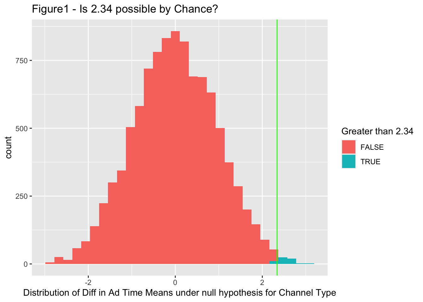
The observed statistic 2.34 is also shown; the fraction of the distribution to the right of that value (≥ 2.34) is the probability that random labeling would give a difference that large. In this case, the probability of this value ( area coloured in green ) is < 0.005.
It would be rare for a difference this large to occur by chance. We have randomly tried “all possible chances” and are hardly able to achieve similar, and the rarer something is, the more likely that there is an underlying truth.
And therefore we conclude there is a real difference between the groups and that ad time is different between
basicandextendedTV channels.
Data Analysis-2: Creating Parallel Worlds
- We will execute on Permutation Test on one sheet step by step and decide whether that factor had a significant effect on STM scores.
- We pretend that there is no difference in scores whether the factor is chosen on way or another.
- We mechanize this pretence by lumping “both kinds” of scores together and shuffle them and divide them, randomly into two groups, and take the difference in scores.
- We can do this, like we did with our Monte Carlo experiment, many many times and calculate difference in scores each time. (It is like inventing many parallel worlds)
- If we look at the way these randomly computed scores are distributed and compare with the one measurement we did see, we can decide whether Mother Nature is up to something, or we are able to mimic the Mom.
- If we are not able to mimic Mom, then Mom always knows and we bow to her and ascribe a significance to the factor under consideration. Else, nope.
- Replicate this test for the other (binary) factors.
Apropos: how could we do this for non-binary factors …??!!!
Making a Data Comic out of our Experiment
What have been our Conclusions with the Experiment? Let us take our Experiment and make a comic out of it:
Data Comic Generator from Gramener (Weblink)
References
Seeing Probability Theory: A Superb visual website to see patterns in theory! Go and play there with Hamlet! (Web Link)
Sampling and Survivourship Bias: Abraham Wald and the Story of WW2 Fighter Planes. (Web Link)
Scientific Method, Statistical Method and the Speed of Light by R. J. MacKay and R. W. Oldford (Web Link)
The Man Who Invented Modern Probability - Andrei Kolmogorov (Web Link)
Tim C. Hesterberg (2015) What Teachers Should Know About the Bootstrap: Resampling in the Undergraduate Statistics Curriculum, The American Statistician, 69:4, 371-386, DOI: 10.1080/00031305.2015.1089789. Available Online (Web Link)
Karan Kashyap, Calculating the Value of Pi: A Monte Carlo Simulation, https://www.cantorsparadise.com/calculating-the-value-of-pi-using-random-numbers-a-monte-carlo-simulation-d4b80dc12bdf
Mahashweta Devi, The Why Why Girl, https://www.tulikabooks.com/picture-books/the-why-why-girl-english.html, read by Sarah Dryden Peterson https://www.youtube.com/watch?v=xNcV5DZhg4c
Fun Stuff: Words Belong Hamlet
Hamlet’s To be or not to be in Pidgin English - Video on FB
To be or Not to be, in Tok Pisin:
`Which way this time? Me killem de finish body b’long me. Or me no do ‘im? Me no savvy.
Might ’e better ’long you-me catchem this fella, string for throw ’im this fella arrow.
Altogether b’long number one bad fella, name b’long him fortune? Me no savvy.
Might ’e better ’long you-me For fightem ’long altogether where him ’e makem you-me sorry too much.
Bimeby him fall down die finish? Me no savvy.’
William Blake, Auguries of Innocence, https://www.poetryfoundation.org/poems/43650/auguries-of-innocence↩︎
Arvind V.
My research interests are Complexity Science, Creativity and Innovation, Problem Solving with TRIZ, Literature, Indian Classical Music, and Computing with R.